xcorr

Unbiased correlation between two complex vectors.

Namespace: dsp::fourier

Prototype

auto xcorr(const Veccf &x, const Veccf &y=Veccf(), int m=-1)

Parameters

x	First vector
y	Second vector (if not specified, the auto-correlation is computed)
m	Number of delays to be computed (if negative, then take \(m=N\)).

Returns

First vector: index of time lags \(n\) (that is \(0, 1, ..., N-1\)), second vector: \(c_n\).

Description

Compute the correlation between 2 complex vectors (through FFT), that is, for negative lags ( \(\tau=-(m-1)\dots -1\)) : \[ c(\tau) = \frac{1}{N-\tau} \cdot \sum_{k=0}^{N-1-\tau} x_{k-\tau} y^{\star}_k \] And, for positive lages ( \(\tau=0\dots m-1\)): \[ c(\tau) = \frac{1}{N-\tau} \cdot \sum_{k=0}^{N-1-\tau} x_k y^{\star}_{k+\tau} \]

Lags are sampled uniformly between \(-(m-1)\) et \(m-1\) : \[ \tau = \textrm{linspace}(-(m-1), m-1, 2m-1) = -(m-1), -(m-2), \dots, -1, 0, 1, \dots, (m-2), (m-1) \]

Note

The vectors are implicitly zero-padded so as to be able to compute efficiently the correlation in the frequency domain.

Example


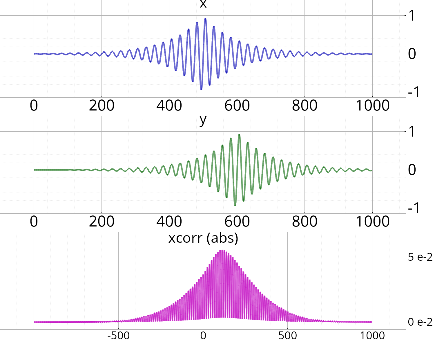
  soit x = sigsin(0.04, 1000) * exp(-abs(linspace(-5,5,1000))),
       y = délais(x, 100);
  soit [lags, c] = xcorr(x, y);

  Figures f;
  f.subplot().plot(x, "b-", "x");
  f.subplot().plot(y, "g-", "y");
  f.subplot().plot(lags, abs(c), "m-", "xcorr (abs)");