Sampling

• Examples
• / Sampling

This little example illustrates the frequency aliasing phenomenum. For this, we sample two simple sinusoïds of different frequencies.

/*  @param fe Fréquence d'échantillonnage
 *  @param sigs Vecteur de spécifications pour signaux sinuisoidaux (fréquences et phases) */
Figure exemple_echan(float fe, const vector<EchanExemple> &sigs)
{
  Figure figure;

  // Parcours les 2 signaux
  pour(auto &s: sigs)
  {
    // Fréquence d'échantillage :
    // soit celle sélectionnée,
    // soit une plus importante pour simuler le signal à temps continu.
    pour(auto f: {fe, 1.0e4f})
    {
      string coul = (&s == &sigs[0]) ? "b" : "r";
      soit t = intervalle_temporel(1.0f, f),
           x = sin(2*π*s.fs*t+s.φ);
      figure.plot(t, x, coul + ((f == fe) ? "o" : "-"));
    }
  }
  retourne figure;
}

Let us begin with two sinusoïds with frequencies 10.5 Hz apart:

exemple_echan(10, {{3}, {13.5}}).afficher();

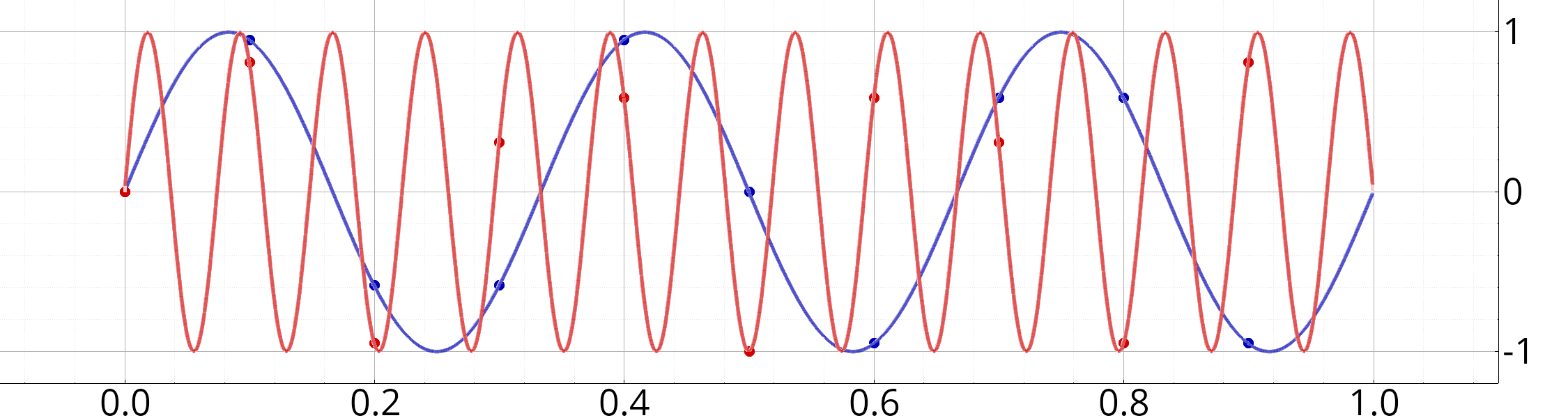
Sampling frequency: 10 Hz, frequency of the two signals: 3 and 13.5 Hz.

The red and blue circles are the samples values. Note that the values of the two signals after sampling are different: it is thus still possible to make a distinction between the two. Now, let us change the frequency of the second signal such as the two frequencies are exactly 10 Hz apart (that is, the sampling frequency):

exemple_echan(10, {{3}, {13}}).afficher();

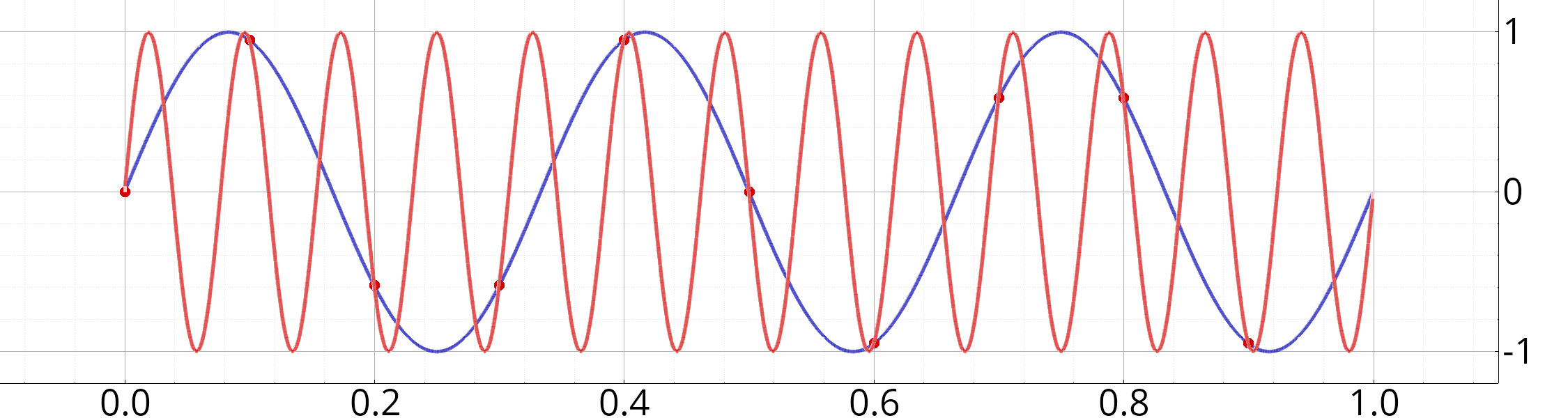
Sampling frequency: 10 Hz, frequency of the two signals: 3 and 13.0 Hz.

Note that, this time, the two signals, after sampling, are no more distinguables.